We LOVE Excel! And, we love it even more when we find a new way to use it to save time and get us results faster. If you have an Excel file with colored cells to sort various information and you’d like to sum the figures in each color group, here’s a quick guide:  

 

Three Quick Steps to Sum by Color in Excel

1. Define the color of the cells using VBA (Visual Basic for Applications)¹

• • Press Alt + F11 keys to enable the Microsoft Visual Basic for Application window.
  • Click Insert > Module to open a new Module
  • In that new module, paste this info:

Function getRGB1(FCell As Range) As String

‘UpdatebyExtendoffice20170714

    Dim xColor As String

    xColor = CStr(FCell.Interior.Color)

    xColor = Right(“000000” & Hex(xColor), 6)

    getRGB1 = Right(xColor, 2) & Mid(xColor, 3, 2) & Left(xColor, 2)

End Function

• • Hit Save and then exit the VBA window.
  • Save the .xls file as an “Excel Macro-Enabled Workbook” now as well
  • This step created a custom formula in Excel that will pull back a unique color identifier/name/classification.

2. Add the color classification to your data

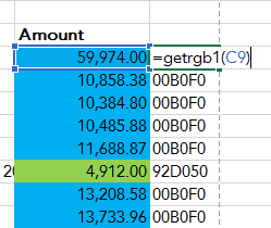
• • Say your colored data starts in column C9; therefore, in column D9, add the formula “=getrgb1(c9)”
  • This will return the “color classification” for that color
  • For example, as shown below, the blue colored cells have a color classification of “00B0F0”
  • Drag this formula down to apply to all your colored cells

3. Now use the “SUM IF” function to return a total by colored cell

• • In the example above, there are two color classifications. To see the total of all the blue cells and all of the green cells, follow the steps below.
  • Assume the amounts we want to total are found in rows 9 to 100.
  • Wherever you’d like the summary of your data to exist, add a couple cells for “Sum of Blue”, “Sum of Green”, etc.
  • Enter this formula next to the “Sum of Blue” cell:
    • =SUMIF(D9:D100,”00B0F0″,C9:C100)
    • This formula is looking at the range of data in Column D, rows 9-100. If the value in those cells is “00B0F0”, the sum the values in Column C, rows 9-100.
  • Enter this formula next to the “Sum of Green” cell:
    • =SUMIF(D9:D100,”92D050″,C9:C100)
    • This formula is looking at the range of data in Column D, rows 9-100. If the value in those cells is “92D050”, the sum the values in Column C, rows 9-100.
  • The result would look something like this:

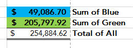
This example was basic but provides the general idea for how to perform Excel functions by a group of cells based upon color.  While a sum function was explained here, a multitude of other Excel functions (AVERAGEIF, COUNTIF, IF, VLOOKUP, etc.) could be applied using the foundation of defining the color and using that as a building block for other functions. 

Written by: Shauna Huntington